![[object Object]](/_next/image?url=https%3A%2F%2Fcdn.sanity.io%2Fimages%2Fei1axngy%2Fproduction%2Fe21406046c81774a7958931b9d4156cf07de0987-460x460.jpg&w=256&q=75)
by Dr Mikkel Lykkegaard
Updated 8 February 2023
DaFT: DerivAtive-Free Thinning
![[object Object]](/_next/image?url=https%3A%2F%2Fcdn.sanity.io%2Fimages%2Fei1axngy%2Fproduction%2F994e45167476c6a2effc9065e5889e96ad8e9b71-600x588.png&w=2048&q=75)
Data thinning, core subset selection, and data compression are critical but often overlooked techniques in data science, machine learning and data-driven science and engineering. When executed correctly, they can lead to massive speed-ups of your analytics pipeline.
In this article, we will unpack these topics, show a few clever tricks, and demonstrate how these ideas can be seamlessly integrated into your existing machine-learning workflow.
Introduction
Data thinning is a problem that arises in multiple different contexts in data science and uncertainty quantification. Perhaps you want to fit a particular model to some data, but your dataset is huge, and your model happens to scale poorly with the size of the dataset. A good example is when building a Gaussian Process surrogate model. Or, perhaps you have many thousands of posterior MCMC samples that you want to run through a (more expensive) model, as illustrated in the figure below.
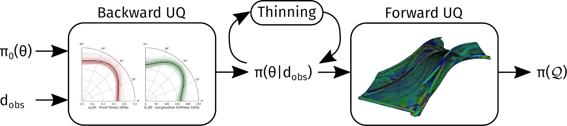
Image sources: Papadimas and Dodwell (2021), The Alan Turing Institute
In such cases, we would like to select an appropriate subset of the data to proceed with, and we refer to this selection process as "thinning". However, the problem can be formulated in multiple other ways:
- Choosing a core subset of the dataset.
- Achieving optimal compression of the data.
The data science team at digiLab has developed a new, lightweight data thinning method (Papadimas et al., 2023) and implemented it in the open-source Python library DaFT. We present here a brief overview of the algorithm and the software library. You can also check out the video and the slides of a presentation that I recently gave at the Workshop on "Multilevel and multifidelity sampling methods in UQ for PDEs" at the ESI Institute at Universität Wien.
To express the problem a bit more formally, consider having a dataset , distributed according to some distribution . We refer to as our empirical distribution. How the data has been generated is not important in this context; could be a Bayesian posterior (when thinning MCMC samples) or the distribution of a physical data-generating process, e.g. sensor output. The problem is then to choose a subset with and "close to" . The first question is then, what do we mean by "closeness"?
Closeness
In this section, we explore the concept of distance between empirical distributions. Feel free to skip ahead if you are more interested in applications than the underpinning theory.
One way to describe the distance between two empirical distributions and is by Maximum Mean Discrepancy (MMD). Consider a feature map where is a Reproducing Kernel Hilbert Space (RKHS). Then the MMD can be defined as (see e.g. Gretton et al., 2012):
For example, if simply , MMD measures the distance between the means of and . If , we also manage to capture the distance between their second moments, that is, their variances, and so on. However, we can make the feature space much richer by using the kernel trick , like so:
The kernel, however, can be very computationally costly to actually compute, particularly for large, high-dimensional datasets. Following Rahimi and Recht (2007), the data can instead be pushed through a random feature map to a Euclidean inner product space, where the inner product approximates the kernel:
Some popular shift-invariant kernels can be approximated by
For example, for a Gaussian kernel we use and .
We then have
which is cheap to compute. While this MMD is only exact for an infinite-dimensional feature space , we are not that interested in the absolute MMD as such, since essentially what we want is to do is find some subset that minimises it.
Minimising the MMD
We are now faced with the optimisation problem of finding a subset of our dataset that minimises the MMD with respect to :
This problem amounts to choosing indices of that best reproduce the empirical distribution of . It is a discrete optimisation problem with possible states and possibly many near--optimal solutions.
This is the type of optimisation problem that is very easily tackled by Genetic Algorithms (GA). In the DaFT software package, we use the excellent open-source Python library DEAP.
Broadly, at generation we initialise a population of candidates ("chromosomes") with size . For each generation , pairs of chromosomes will be chosen at random, and their genes will be randomly swapped ("mating"). Similarly, single chromosomes will be randomly chosen and randomly perturbed ("mutation"). The fitness of each chromosome is then evaluated using the fitness function . Finally, the fittest chromosomes will be moved to the next generation by way of some selection criterion. For more details on Genetic Algorithms, see e.g. Mitchell (1998).

Genetic Algorithm
Repeating this process for sufficiently many generations will yield an optimal subset , which, given the heurestic nature of GA, may not be the most optimal subset. However, it is many orders of magnitude cheaper to find than the exact optimum, and for most intents and purposes it doesn't matter.
Examples using DaFT
Example 1: Banana
Consider the banana distribution, were the normally distributed random variables are transformed through the following map:
Our complete dataset consists of samples from this dataset and we are interested in extracting a subset of . We could achieve that by just drawing random indices uniformly:
n_sub = 20
Y_random = X[np.random.randint(X.shape[0], size=n_sub), :]
Using DaFT, we could instead employ optimal thinning of the dataset to produce a core set:
daft = DaFT(X, n_sub)
Y_best, _ = daft.run(n=500, ngen=200)
Plotting the complete dataset along with the two different subsets, we get the following:
plt.figure(figsize=(6,4))
plt.scatter(X[:,0], X[:,1], alpha=0.1, c='k')
plt.scatter(Y_random[:,0], Y_random[:,1], alpha=1, c='tomato')
plt.scatter(Y_best[:,0], Y_best[:,1], alpha=1, c='springgreen')
plt.show()
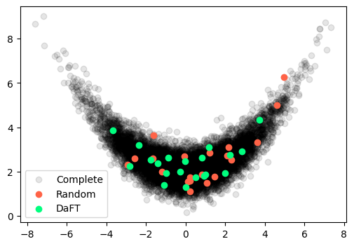
Banana Distribution
In this case, the simple random sampler has oversampled the right tail of the distribution and missed out on the left tail, while DaFT has covered the entire distribution.
Example 2: Gaussian Blobs
In this example, we consider nine Gaussian blobs with different means and samples for the complete dataset . Note that the central blob has twice as many samples as the others. For our subset , we now select samples from the complete dataset.
Using the exact same approach as outlined above, we get the following output:
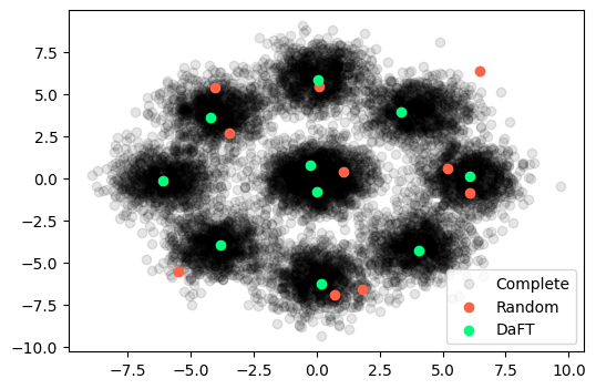
Gaussian Blobs
In this case, the simple random sampler has completely missed some of the blobs, while DaFT has taken a single sample from the centre of each of the peripheral blobs and two samples from the central blob, which contains twice as many samples as each of the other blobs.
The Reading
-
A. Gretton, K. M. Borgwardt, M. J. Rasch, B. Schölkopf, A. Smola, A Kernel Two-Sample Test, 2012, Journal of Machine Learning Research.
-
M. Mitchell, An Introduction to Genetic Algorithms, 1998, The MIT Press.
-
N. Papadimas, M. B. Lykkegaard, T. J. Dodwell, Derivative-Free Thinning (DaFT) with Stochastic Kernel Embeddings, 2023, Manuscript in Preparation.
-
A. Rahimi, B. Recht, Random Features for Large-Scale Kernel Machines, 2007, Advances in Neural Information Processing Systems.
About digiLab
digiLab is an agile, deep tech company operating as a trusted partner to help industry leaders make actionable decisions through digital twin solutions. We invent first-of-a-kind, world-leading machine learning solutions which empower senior decision-makers to exploit the value locked in their data and models.
Featured Posts
If you found this post helpful, you might enjoy some of these other news updates.
Python In Excel, What Impact Will It Have?
Exploring the likely uses and limitations of Python in Excel

Richard Warburton
Large Scale Uncertainty Quantification
Large Scale Uncertainty Quantification: UM-Bridge makes it easy!

Dr Mikkel Lykkegaard
Expanding our AI Data Assistant to use Prompt Templates and Chains
Part 2 - Using prompt templates, chains and tools to supercharge our assistant's capabilities

Dr Ana Rojo-Echeburúa